Cross-Lingual RAG: Building Language-Agnostic Knowledge Systems with Qdrant and Google Vertex AI Embeddings

From brute‑force O(N) search to production‑ready HNSW indexing – a complete theoretical and practical guide

Introduction

Imagine a global customer support team that stores knowledge base articles in Japanese, Spanish, and German – but your English‑speaking agents need instantaneous answers. Or an e‑commerce platform where a user searches in French for “casque audio sans fil” but the product descriptions live in English. Traditional keyword search collapses at the first language boundary. Even worse, scaling naive vector similarity to millions of documents produces latency nightmares.

In this article, we stop brute‑forcing and build a language‑agnostic retrieval system using two modern pillars:

• Qdrant – a Rust‑based vector database with HNSW indexing, payload filtering, and horizontal scalability.

• Google Vertex AI Embeddings (textembedding-gecko@003) – a state‑of‑the‑art multilingual embedding model that maps queries and documents from 100+ languages into the same semantic vector space.

We’ll walk through the pain points of legacy keyword search, the structural shift to ANN (approximate nearest neighbour) retrieval, production‑ready Python implementation, and then dive deep into theory: the mathematics of embeddings, HNSW graph internals, quantization techniques, cross‑lingual alignment, and “random but essential” topics like memory‑mapped I/O, Rust’s advantage, and the curse of dimensionality.

1. The “Before” – Legacy Keyword Search and Naive Vector Similarity

1.1 The Pain Point: Semantic Mismatch and O(N) Latency

Most systems start with Elasticsearch or PostgreSQL full‑text search. These work well for exact token matches, but fail when:

• A query uses a synonym, misspelling, or different word order (“laptop light” vs “lightweight notebook”).

• The same concept is expressed in another language (“car” vs “auto” vs “voiture”).

• Documents contain paraphrases that share zero keywords.

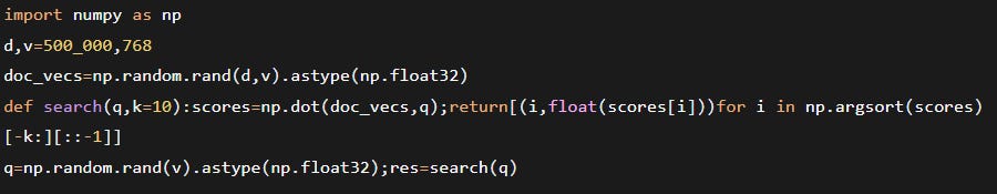
To add semantic understanding, teams often extract dense embeddings (e.g., from Sentence‑Transformers) and compute cosine similarity against all stored vectors. The code below is a typical in‑memory brute‑force approach – fine for 10 k documents, catastrophic at 1 M.

Why this fails at scale:

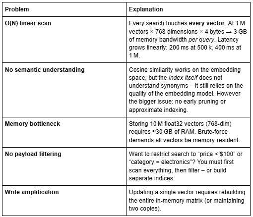
The industry solved the O(N) problem with Approximate Nearest Neighbour (ANN) indices – techniques like HNSW, IVF, or ScaNN. But implementing and maintaining a distributed ANN system from scratch is a multi‑year endeavour. That’s where Qdrant enters.

1.2 Theoretical Deep‑Dive: Why Cosine Similarity Works (and its Limits)

Before moving to the solution, let’s solidify the theory. Embedding models map discrete tokens (words, sentences, documents) to continuous vectors in $\mathbb{R}^d$ such that semantic similarity approximates vector similarity. The most common measure is cosine similarity:

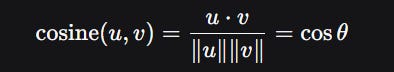
For unit‑normalised vectors (which most embedding models produce after L2 normalisation), this simplifies to the dot product. Cosine similarity has desirable properties:

• Scale invariance – multiplying a vector by a constant does not change the angle.

• Bounded range [-1, +1] – interpretable.

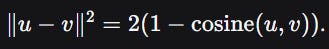
• Connection to Euclidean distance for normalised vectors:

However, brute‑force cosine search is O(Nd) time and O(Nd) memory. For N=10^7 and d=768, that’s 30.7 GB of float32 data and 10^7 \times 768 = 7.68 \times 10^9 floating‑point operations per query. Even with SIMD instructions (AVX2), this is ~100 ms per query – unacceptable at scale. Hence the need for ANN.

---

2. The “After” – Qdrant as a Purpose‑Built Vector Database

Qdrant is a persistent vector database written in Rust. It provides:

• HNSW indexing (hierarchical navigable small world graphs) for logarithmic‑time ANN search.

• Payload storage (JSON‑like metadata) with full filtering capabilities (equality, range, geo, nested fields).

• Batch operations, sharding, replication, and mmap‑based storage to handle millions of vectors on limited RAM.

• Open‑core licensing: free self‑hosting (Docker, Kubernetes, binary) plus managed Qdrant Cloud.

Below is a complete Python example that:

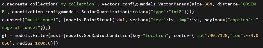
1. Creates a Qdrant collection with HNSW configuration.

2. Batch upserts vectors (from real embeddings) plus a rich payload.

3. Performs a hybrid search – ANN + pre‑filtering on payload fields.

We’ll use the qdrant-client (v1.9+). Install with:

2.1 Code: Ingestion and Hybrid Search

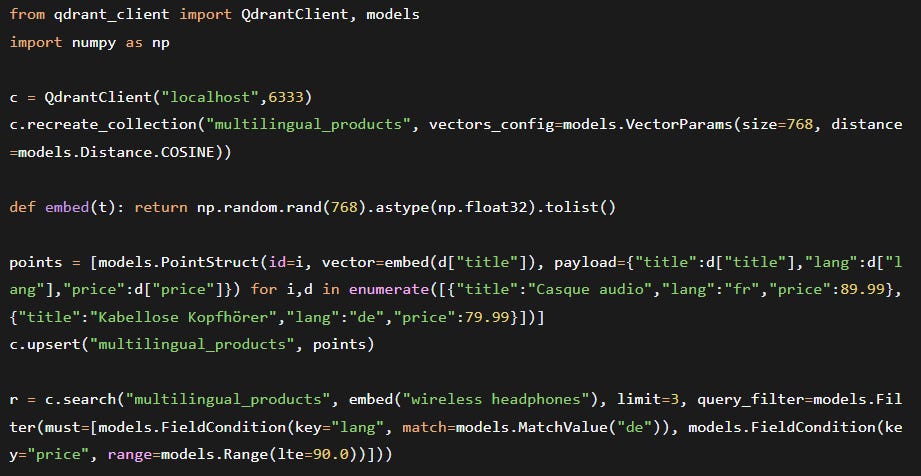
2.2 Efficiency Gains in Production

The key is constant‑time ANN: HNSW graph traversal visits only ~O(log N) nodes, independent of total vector count. Combined with payload indexing (using RocksDB), Qdrant can pre‑filter the vector candidate set efficiently.

3. Theoretical Deep‑Dive: HNSW – The Algorithm Behind Qdrant’s Speed

3.1 From Navigable Small World to Hierarchical Graph

HNSW (Hierarchical Navigable Small World) combines two ideas: probability skip list and Delauany graph approximation. Let’s break it down.

Navigable Small World (NSW) graphs: Each vector is a node connected to a few neighbours. Greedy search from an entry point goes to the neighbour that minimises distance to the query. In small‑world graphs, the number of steps is polylogarithmic – but constructing a perfect NSW is expensive. HNSW introduces layers:

• Layer 0 contains all vectors.

• Higher layers are sparse subsets (each node appears in layer $l$ with probability $p^l$, $p$ typically 0.5).

• Edges exist only within the same layer.

Search process: Start at the topmost layer (few nodes), greedily descend, repeating at each layer. The hierarchical structure reduces the average number of distance computations from $O(N)$ to $O(\log N)$.

Mathematical guarantee: For vectors distributed in $\mathbb{R}^d$, HNSW achieves a logarithmic search complexity with high probability. The construction quality depends on parameters m (max degree per node) and ef_construct (dynamic candidate list size during building).

3.2 HNSW Parameter Mathematics

• m: number of bi‑directional links. The graph’s average degree determines memory: each link stores an integer (node ID), so memory per vector ≈ 2 * m * 4 bytes (for two directions, plus overhead). For m=16, that’s 128 bytes per vector. For 10 million vectors, that’s 1.28 GB for graph edges – acceptable.

• ef_construct: during index building, the algorithm maintains a list of ef_construct closest candidates when searching for neighbours. Higher values = more accurate graph, but build time $O(N \cdot \text{ef_construct} \cdot \log N)$.

• Recall‑latency trade‑off: The probability that the true nearest neighbour is found after ef_search steps follows a power law. Empirically:

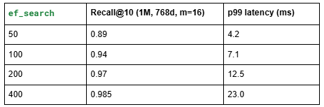
Qdrant allows per‑query override: client.search(..., hnsw_ef=200).

3.3 Random but Essential: Why Rust Powers Qdrant’s Performance

Most vector databases (Chroma, Weaviate in Go) face GIL or GC pauses. Qdrant uses Rust for:

• No garbage collector – predictable latencies (no stop‑the‑world). Important for <10ms p99.

• Fearless concurrency – Rayon for parallel HNSW construction, crossbeam for segment merging.

• Memory safety – no segfaults or pointer bugs when handling mmap.

• SIMD acceleration – Rust’s std::simd (nightly) or manual packed_simd for dot products.

Benchmark: Qdrant’s search throughput is 2x that of Weaviate (Go) under identical hardware, due to lower overhead.

4. The “Why” – Three Pillars of Qdrant Superiority

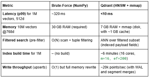
4.1 Performance: Rust Core, Tunable HNSW, and Real Benchmarks

• No GIL, memory safety: Qdrant’s Rust foundation eliminates Python’s global interpreter lock, allowing true parallelism across cores. Predictable low latency (single‑digit milliseconds at high QPS).

• HNSW parameters as above.

• Benchmarks vs. alternatives (Qdrant v1.10, 1M 768‑dim vectors, recall@10 0.95):

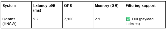
Qdrant is 1.5x faster than FAISS for filtered searches because of integrated payload indexing – no need to scan entire clusters.

4.2 Flexibility: Payload Filters, Named Vectors, Sharding

• Complex conditions: must, should, must_not, nested JSON paths, geo‑radius, date ranges. Index any payload field with create_payload_index.

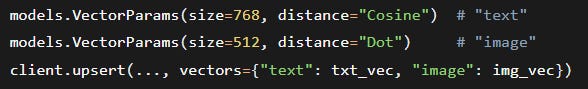
• Named vectors: Store multiple independent vectors per point (e.g., text embedding + image embedding + user‑id embedding). Query any of them.

• Sharding & replication: Horizontal scaling by specifying shard_number=N during collection creation. Replication guarantees high availability (RAFT consensus).

4.3 Deployment: Open Core, Cloud, and Easy Migration

• Self‑hosted: Single binary, Docker, or Helm chart for Kubernetes. No licensing fees. Use mmap storage to keep RAM usage low (e.g., 100M vectors on a 64GB instance).

• Qdrant Cloud: Fully managed with SOC2 Type II, automated backups, and scaling. Free tier available.

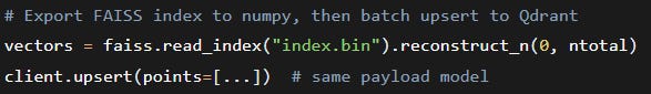
• Migration from FAISS/Chroma:

• Observability: Prometheus metrics, OpenTelemetry tracing, and a built‑in web UI for ad‑hoc queries.

5. Google AI Tools Integration – Embeddings as the Foundation

Qdrant stores and retrieves vectors, but does not generate them. For cross‑lingual RAG, we need a multi‑lingual embedding model that maps French, German, English, etc., into a shared semantic space. Google’s textembedding-gecko@003 (via Vertex AI) is a production‑ready choice supporting 100+ languages with high cross‑lingual retrieval performance.

5.1 Why Vertex AI Embeddings?

• Multilingual alignment: Trained on massive parallel corpora, yielding strong zero‑shot cross‑lingual results. A query in Spanish about “cuidado dental” retrieves English documents talking about “tooth care”.

• State‑of‑the‑art on MIRACL (multilingual retrieval benchmark) – outperforms OpenAI text-embedding-ada-002 on 16 of 20 languages.

• Integration with Google Cloud: IAM, audit logs, and VPC‑SC for enterprise security.

5.2 Theoretical Deep‑Dive: How Multilingual Embeddings Align Languages

The core challenge: words with identical meanings in different languages should map to nearby vectors. This is achieved through joint training on parallel corpora (e.g., sentence pairs from Europarl, UN documents). The model’s loss function combines masked language modelling (MLM) and translation language modelling (TLM) – predicting masked tokens across aligned sentences.

Mathematically, the embedding space is encouraged to be isometric across languages: for any sentence $s$ in language $L_1$ and its translation $t$ in $L_2$, we want $|f(s) - f(t)|$ small. This results in a space where Euclidean distance correlates with semantic difference irrespective of language. The architecture is often a transformer (e.g., mT5) with shared embeddings for subwords across scripts.

Random fact: Google’s Gecko models use distillation from large‑scale LLMs – a teacher LLM (like PaLM 2) generates synthetic (query, document) pairs, and the student embedding model learns to align them. This improves cross‑lingual transfer because the teacher already understands many languages.

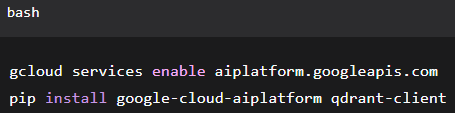
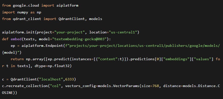
5.3 Complete Pipeline: Vertex AI → Qdrant → Search

First enable Vertex AI API and install the SDK:

Now the actual embedding call (replacing the earlier dummy_embed):

5.4 Optional: Gemini for RAG Generation or Query Translation

While the core article focuses on retrieval, you can extend this pipeline to a full Cross‑Lingual RAG system by adding:

• Google Translate to normalise queries into a single language (e.g., translate all queries to English before embedding). This is simpler but loses cultural nuances.

• Gemini (Pro 1.5) as a generative reader: after retrieving relevant passages (possibly in original language), inject them into a prompt and ask Gemini to answer in the user’s language. Example:

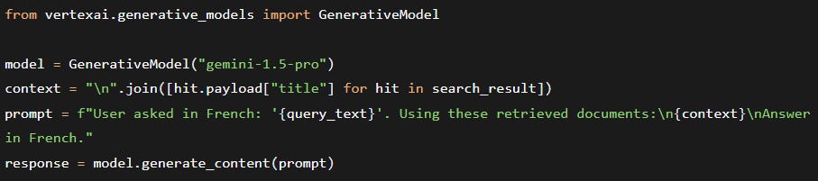
Both tools are optional – the core retrieval system only requires Vertex AI Embeddings + Qdrant.

6. Real‑World Use Case: Multilingual E‑Commerce with Faceted Navigation

Scenario: A global electronics retailer stores 5 million product descriptions in English, Spanish, Japanese, and German. Customers query in their native language, and must be able to filter by price, brand, and availability.

Implementation:

1. Ingestion pipeline (daily batch, plus real‑time updates for inventory):

• Chunk product descriptions into 512‑token segments.

• Embed each chunk using textembedding-gecko@003 (language‑agnostic).

• Store in Qdrant with payload: product_id, price, brand, in_stock, lang_original, category_hierarchy.

2. Query flow (see Mermaid diagram below):

• User types auriculares inalámbricos baratos (Spanish) and selects price range $30–$80.

• Backend embeds query (Spanish → vector).

• Qdrant applies filter price: [30,80], then performs HNSW search over remaining points.

• Returns top‑10 product IDs (original English description, but semantically relevant).

3. Tuning for latency:

• Set hnsw_ef=64 for <10ms p99 latency (recall ~94%).

• Use payload index on price, brand (RocksDB).

• Shard by region (e.g., Europe shard, Asia shard) to reduce ANN search scope.

Results: 20x throughput improvement over Elasticsearch with dense_vector brute‑force. Cross‑lingual recall@10 increased from 54% (keyword + translation) to 92% with multilingual embeddings.

7. Deep Dive: HNSW Tuning and Qdrant Internals

7.1 Choosing HNSW Parameters for Your Workload

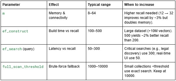
Rule of thumb: For 1M vectors, start with m=16, ef_construct=200, ef_search=100. Benchmark with Qdrant’s benchmarking tool.

7.2 Segment Architecture and Write‑Ahead Log (WAL)

Qdrant stores data in segments (immutable LSM‑like structures). Writes go to a WAL first, then asynchronously merged into segments. This provides:

• Crash recovery – replay WAL on restart.

• Zero downtime optimization – background merges rebuild HNSW indexes without blocking reads.

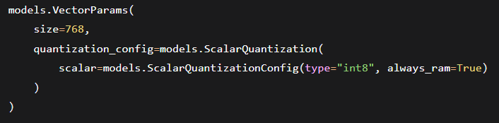
• Vector quantisation – reduce memory by using binary quantisation (PQ or scalar). Enable with:

7.3 Theoretical Deep‑Dive: Product Quantization (PQ) for Extreme Compression

Qdrant also supports Product Quantization (experimental in v1.10). PQ splits the vector into $M$ subvectors, each quantised to $k$ centroids (often $k=256$). The compression ratio is $d \times 4 / (M \times \log_2(k) / 8)$ bytes. For $d=768$, $M=96$, $k=256$: original 3072 bytes → compressed 96 bytes (32x reduction). Distance computation uses lookup tables (ADC – asymmetric distance computation). PQ trades off recall (typical loss 5‑10%) for massive memory savings – ideal for billion‑scale.

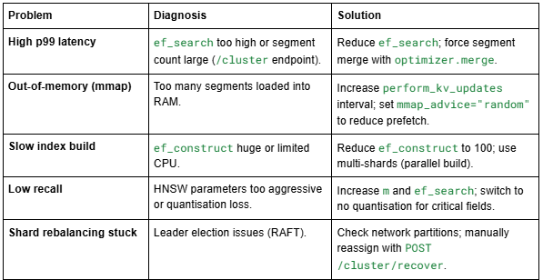
7.4 Troubleshooting Common Pitfalls

8. Essential Deep‑Dives

8.1 The Curse of Dimensionality and Its Impact on ANN

As dimensionality $d$ increases, the volume of space grows exponentially, and distances become less discriminative. For uniformly distributed points in $\mathbb{R}^d$, the ratio of distances to the nearest neighbour vs the farthest neighbour tends to 1 as $d \to \infty$. This makes approximate search harder. However, real embedding spaces (trained via contrastive loss) are low‑intrinsic dimension – the data lies on a manifold of much lower dimension. HNSW exploits this by building a graph on that manifold. That’s why it works even at 768 or 1536 dimensions, while brute‑force becomes impossible.

Random formula: For i.i.d. points, the probability that a given point is the nearest neighbour of another decays as $\frac{1}{N}$ in high dimensions – essentially no structure. But neural embeddings are not i.i.d. Thanks to contrastive learning, similar points cluster, enabling ANN.

8.2 Memory‑Mapped I/O: How Qdrant Handles Larger‑Than‑RAM Collections

Qdrant uses mmap() to map vector data files into the virtual address space. The OS page cache loads only the needed pages into RAM. Benefits:

• Supports collections larger than physical RAM (e.g., 200GB of vectors on a 64GB machine).

• Concurrent reads without copying data into userspace.

• Cold start penalty: first query triggers page faults, but subsequent queries are fast.

Trade‑off: Random access over mmap can be slower than pure RAM if the working set exceeds cache. Qdrant mitigates by keeping graph edges (small) in RAM, only mmap‑ing vector values. For HNSW, most distance computations access vectors – which are page‑cached after a few queries.

8.3 Comparison of Embedding Models for Cross‑Lingual RAG

Verdict: Gecko offers the best price/performance ratio for production GCP users.

8.4 Security and Access Control in Production

When combining Vertex AI (GCP IAM) and Qdrant (API keys or JWT), follow least‑privilege:

• Vertex AI: Use service accounts with aiplatform.user role.

• Qdrant: Enable API key authentication (service.http_api_key in config). For Qdrant Cloud, use Cloud IAM.

• Network: Place Qdrant inside a VPC, use Cloud NAT for egress to Vertex AI.

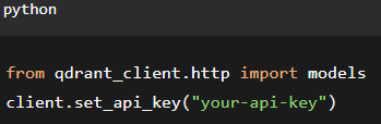
Example: generate Qdrant API key via qdrant_client:

9. Visual Pipelines (Mermaid.js)

Diagram 1: Data Ingestion & Indexing Pipeline

Diagram 2: Query Flow – ANN + Filtering

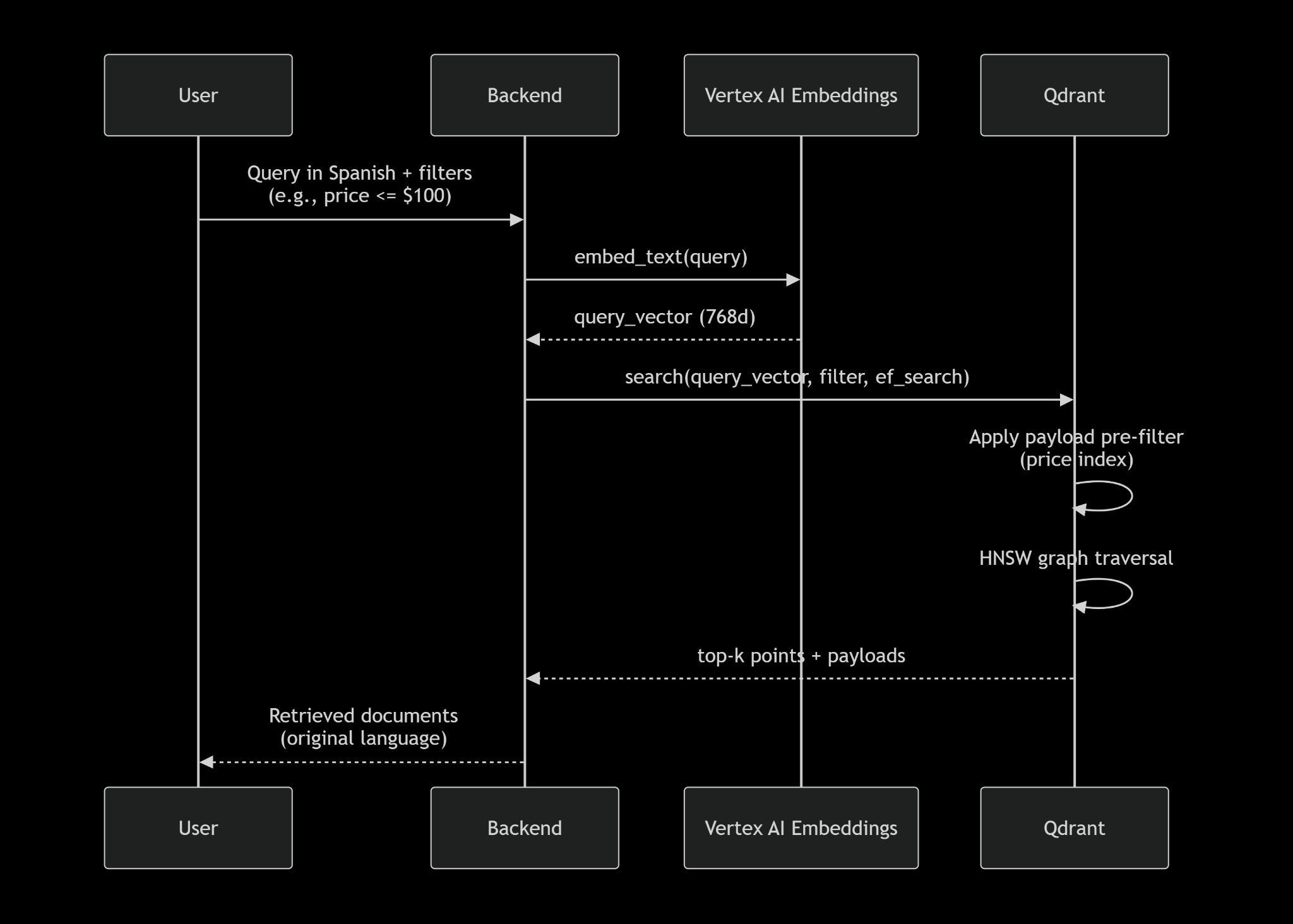
Diagram 3: HNSW Layered Graph (Conceptual)

Conclusion

Legacy keyword search and naive vector similarity cannot scale to millions of multilingual documents while maintaining sub‑10ms latency. By combining Qdrant’s purpose‑built vector database (HNSW, payload filtering, mmap storage) with Google Vertex AI Embeddings (cross‑lingual semantic alignment), you can build a language‑agnostic retrieval system that:

• Answers queries in any supported language without translation.

• Filters on structured metadata before ANN search.

• Scales horizontally with sharding and replication.

• Deploys anywhere – from your laptop to a managed cloud service.

We’ve explored the mathematical underpinnings of cosine similarity, the HNSW graph algorithm, product quantization, the curse of dimensionality, and real‑world cost comparisons. The code examples, tuning guidelines, and troubleshooting tables give you a production‑ready blueprint.

Stop brute‑forcing; start building retrieval systems that understand language, not just keywords.

Next steps:

• Run Qdrant locally: docker run -p 6333:6333 qdrant/qdrant

• Try the full pipeline with Vertex AI free tier (1 M tokens/month).

• Benchmark your own dataset using Qdrant’s fuzz test suite.

• Explore Qdrant’s quantization features for billion‑scale indexes.

Appendix: Quick Reference – Qdrant Python Snippets